Bottleneck Theory of Post-training

This is the inaugural post of a blog I have wanted to start for some time. It is a great opportunity to begin with a topic I enjoy. I wrote it together with Fabio Valerio Massoli, following our upcoming NeurIPS 2026 paper on conditional information bottleneck methods for neural reasoning.

In modern reasoning-model training, we hear of methods like RL with verifiable rewards (RLVR) [1], reinforcement learning from AI feedback (RLAIF) [2], on-policy distillation (OPD) [3], on-policy self-distillation [4], and many other variants. They differ in where their training signal comes from, whether the signal is scalar or token-level, and whether the training data are on-policy or offline. Despite the differences, they optimize remarkably similar objectives.

This is the main message of this post and of our paper Reasoning as Compression [5]:

Reasoning models learn a stochastic reasoning channel that simulates a path from question to answer, with reasoning structure emerging from constraints on that path. Post-training methods are special cases of this view, formalized through the conditional information bottleneck framework.

In particular, budget-forcing variants [6], which compress reasoning tokens, are a special case of the bottleneck view: reasoning traces should preserve task-relevant information while discarding information that is unnecessary, costly, or already available from the prompt.

We introduced the Conditional Information Bottleneck (CIB) in our paper Reasoning as Compression: Unifying Budget Forcing via the Conditional Information Bottleneck [5] to formalize this view.

Reasoning, the information bottleneck, and the emergence of structure

What is reasoning? There are many accounts of reasoning, but let’s start with this one: “Theoretical reasoning is a mental process that takes you from premises that you believe to a conclusion that you come to believe as a result of the process” (Broome, 2021 [7]).

We can look at neural reasoning in a similar way: as a process, a path from a premise (the prompt or query) to a conclusion (the final answer). The differences between post-training methods can be organized within a single information-theoretic picture:

Reasoning is about learning to simulate a stochastic channel that takes the prompt to the final answer.

Of course, human reasoning also has normative features, including adherence to inference rules, logical consistency, evidence accumulation, and attribution. The hope is that post-training can help these structures emerge through learning, without necessarily encoding the rules directly in the model.

The emergence of structure under constraints is a recurring theme in physics, information theory, complexity theory, and biology. We will use the information bottleneck framework (Tishby, Pereira, and Bialek, 1999 [8]), which has also been applied to deep learning (Shwartz-Ziv and Tishby, 2017 [9]). In information bottleneck, given a joint distribution between an input variable \(X\) (the data) and a relevant target variable \(Y\) (what needs to be predicted), we want to find a compressed representation \(T\) that retains as much information about \(Y\) as possible. The constraint is on \(T\): the mutual information \(I(X; T)\) needs to be constrained. In this case, optimizing the Lagrangian \(\mathcal{L} = I(T; Y) - \beta I(X; T)\) forces the system to perform a non-linear quantization. Irrelevant information and noise in \(X\) are stripped away. What remains is a parsimonious, maximally informative sufficient statistic (\(T\)) that captures the structure needed to solve the problem.

To apply the information bottleneck to reasoning, there is a catch.

Conditional information bottleneck

Consider a reasoning problem with

\[X \sim P_{\mathcal D}(X), \qquad Y \sim P_{\mathcal D}(Y\mid X),\]

where \(X\) is the user/problem prompt and \(Y\) is the desired answer.

A reasoning model samples an intermediate trace

\[Z=(z_1,\ldots,z_T)\sim \pi_\theta(\,\cdot\mid X),\]

and then produces an answer according to

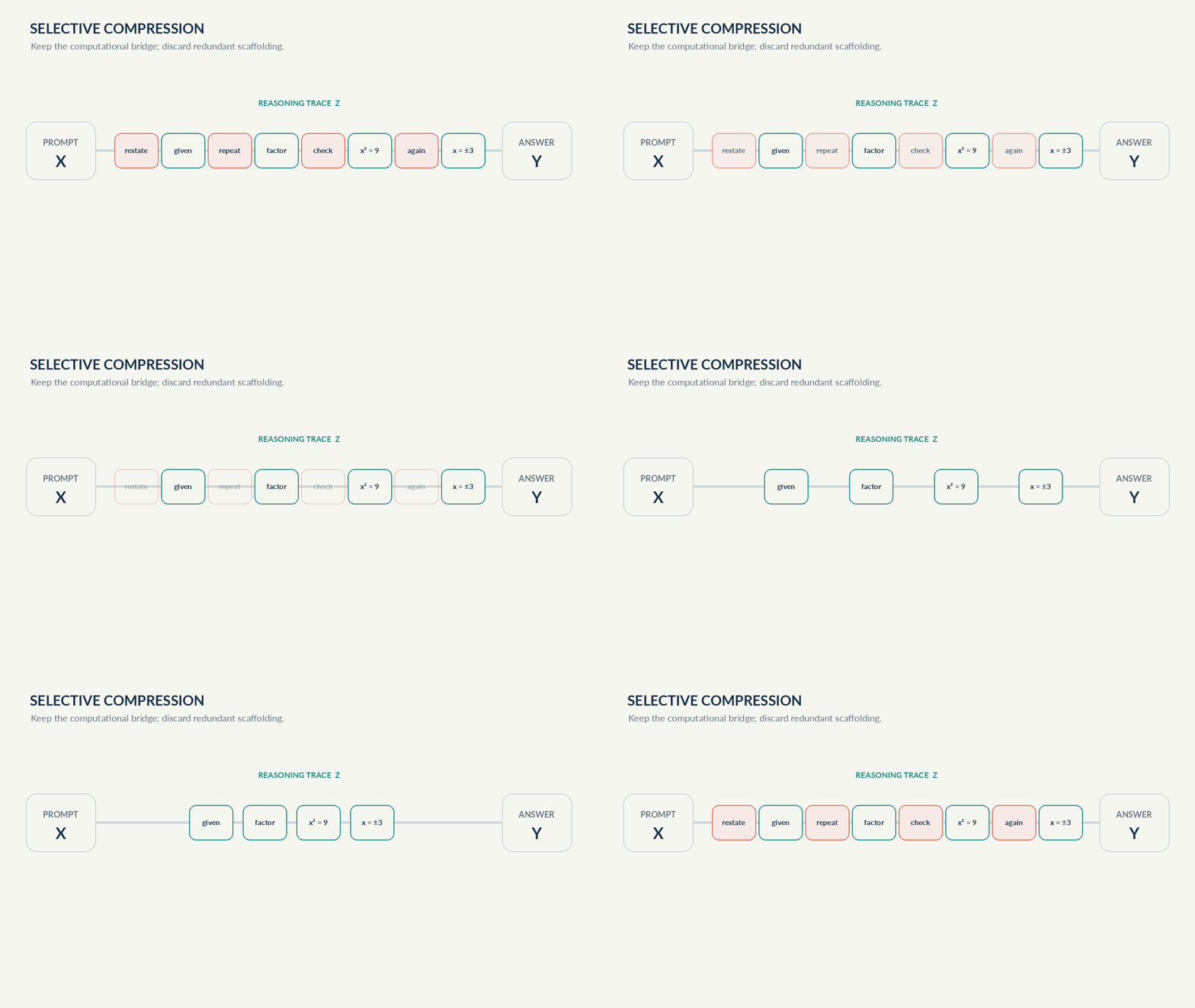
\[\pi_\theta(Y\mid X,Z).\]

The usual intuition is that \(Z\) is a computational bridge: it contains information that helps transform \(X\) into \(Y\). A good reasoning trace should satisfy two apparently opposing requirements:

• Sufficiency: \(Z\) should contain the information about \(Y\) that is useful beyond what is already available from \(X\). This is captured by \(I(Z;Y\mid X)\).
• Minimality: \(Z\) should not contain unnecessary information. This is captured by \(I(X;Z)\).

The corresponding conditional information bottleneck (CIB) is

\[\boxed { \max_{\pi_\theta} I(Z;Y\mid X)-\beta I(X;Z) } \tag{1}\]

where \(\beta\ge 0\) controls the accuracy-compression trade-off. The optimization problem is solved under the condition that the distribution \(\pi_\theta\) satisfies the marginalization condition:

\[\sum_{z} \pi_\theta (y|x,z)\pi_\theta(z|x) = P(Y|X).\]

We will see that this constraint is imposed implicitly through the sampling procedure.

This formulation was introduced specifically to repair a problem with applying the classical Information Bottleneck directly to chain-of-thought [10]. In a transformer, the answer decoder sees both \(X\) and \(Z\); therefore the Markov assumption underlying the ordinary IB,

\[Y\leftrightarrow X\leftrightarrow Z,\]

is not the right structural model. CIB instead asks for information about \(Y\) that is conditional on \(X\).

There are other differences from the classical literature on channel simulation and information bottleneck:

• In information-theoretic setups, the distribution \(P(Y\mid X)\) is known, and the goal is to find a stochastic encoder \(P(Z\mid X)\) and a decoder \(P(Y\mid Z)\). However, in reasoning, we only have access to \(P(Y\mid X)\) through samples \((X_i,Y_i)\), which are reference examples in our dataset.
• In classical information bottleneck, the optimization is over \(P(Z\mid X)\) and \(P(Y\mid Z)\). In the case of neural reasoning, the optimization is over parameters \(\theta\) of a model \(\pi_\theta\).

These differences impact how we optimize and approximate the objective.

Simulating the reasoning channel

For every prompt \(x\), let \(\pi_\theta(z\mid x)\) be the reasoning policy we want to learn. Let’s study each of the two terms.

Minimality: The term \(I(X;Z)\) measures the information we want to minimize to compress \(Z\). It is given by:

\[I(X;Z) =\mathbb E \big(\log\frac{\pi_{\theta}(Z|X)}{P(Z)}\big)\]

The expectation can be estimated empirically using samples of \((X,Z)\), but it still requires knowledge of \(P(Z)\). What is \(P(Z)\) and why does it pop up in the expression? The distribution \(P(Z)\) is a prior over the space of reasoning traces. Intuitively, the term \(P(Z)\) pushes the generated trace \(Z\) toward the space of reasoning traces. In other words, \(\log P(Z)\) in the CIB bound rewards the use of natural reasoning traces. \(P(Z)\) is unknown in general, but we can use any other approximate prior \(Q\) (as in Alemi et al., 2017 [11]) and use this relation:

\[\mathbb E_X D_{\mathrm{KL}} \big( \pi_\theta(z\mid X)\|Q(z) \big) = I(X;Z) + D_{\mathrm{KL}}(P_Z\|Q). \tag{2}\]

Hence:

\[I(X;Z) \le \mathbb E_X D_{\mathrm{KL}} \big( \pi_\theta(z\mid X)\|Q(z) \big). \tag{3}\]

We can therefore minimize the minimality term by minimizing its KL-to-prior upper bound.

Sufficiency: This is the term we want to maximize. We can write \(I(Z;Y\mid X)=H(Y\mid X) - H(Y\mid X,Z)\). The first term \(H(Y\mid X)\) is independent of \(Z\), so we just need to maximize \(-H(Y\mid X,Z)\). A similar variational argument gives a lower bound using any variational decoder \(q_\theta(y\mid x,z)\):

\[\mathbb E_P[\log q_\theta(y|x,z)] = -H(Y|X,Z) - \mathbb E\,\mathrm{KL}\big(p(\cdot|x,z)\,\|\,q_\theta\big)\le -H(Y|X,Z).\]

\(q_\theta\) can be chosen such that \(\log q_\theta(y\mid x,z)\) is any scalar sufficiency signal assigned to a trajectory. It can be a binary verifier reward, a learned reward model, an AI-generated preference score, a teacher’s token-level log probability, a self-teacher’s log probability, a supervised likelihood, or a filtered/weighted version of a supervised target. To maximize the first term in the CIB bound, we maximize the lower bound \(\log q_\theta(y\mid x,z)\).

To impose the marginal probability constraints, note that \(\pi_\theta\) is by design a probability distribution. The marginal probability constraint can be imposed by assuming that each question \(x\) has a unique answer \(y\) and modifying the sampling accordingly.

We are then ready to solve the optimization problem using any chosen sufficiency signal \(\log q_\theta(y\mid x,z)\) and any prior \(Q(z)\):

\[\max_{\pi_\theta} \mathbb E_{(x,y)\sim P_{\textrm{true}},z\sim\pi_\theta(\cdot|x)} \left[ \log q_\theta(y\mid x,z) \right]-\beta \mathbb E_X D_{\mathrm{KL}} \big( \pi_\theta(z\mid X)\|Q(z)\big). \tag{4}\]

The negative KL term can be decomposed as \(\mathbb E_z\log Q(z) + H(\pi_\theta(\cdot\mid x))\). This is a typical entropy-regularized post-training objective with reward \(\log q_\theta(y\mid x,z)\), together with an additional term \(\log Q(z)\) that compresses the traces using the prior \(Q\).

Compressing the reasoning trace

Different budget-forcing methods can be understood as different choices of prior over reasoning traces within the same Conditional Information Bottleneck (CIB) objective. The prior determines what kind of reasoning is considered expensive.

Linear length penalties: uniform prior. Suppose every token has equal probability:

\[Q(z_t)=\frac{1}{|V|}.\]

Then every token has the same information cost, regardless of its meaning:

\[\log Q(Z)=-T\log |V|.\]

Consequently, the CIB objective reduces to a conventional linear length penalty. The implicit assumption is that every additional token is equally expensive.

Target-length forcing: Laplace prior. Consider methods such as LCPO-Exact, which encourage the generated reasoning length to match a target length \(T^\star\). This corresponds to choosing a prior over sequence length:

\[Q(T)\propto \exp(-|T-T^\star|).\]

The resulting log-prior is \(\log Q(T)=-|T-T^\star|+\text{constant}\). In other words, target-length forcing is a CIB objective with a prior that concentrates probability around a preferred reasoning length. It penalizes being too short as well as being too long.

Semantic compression: language-model prior. We propose using a frozen pretrained language model as the prior:

\[Q_\phi(Z)= \prod_{t=1}^{T}Q_\phi(z_t\mid z_{<t}).\]

It gives the following information cost for the trace:

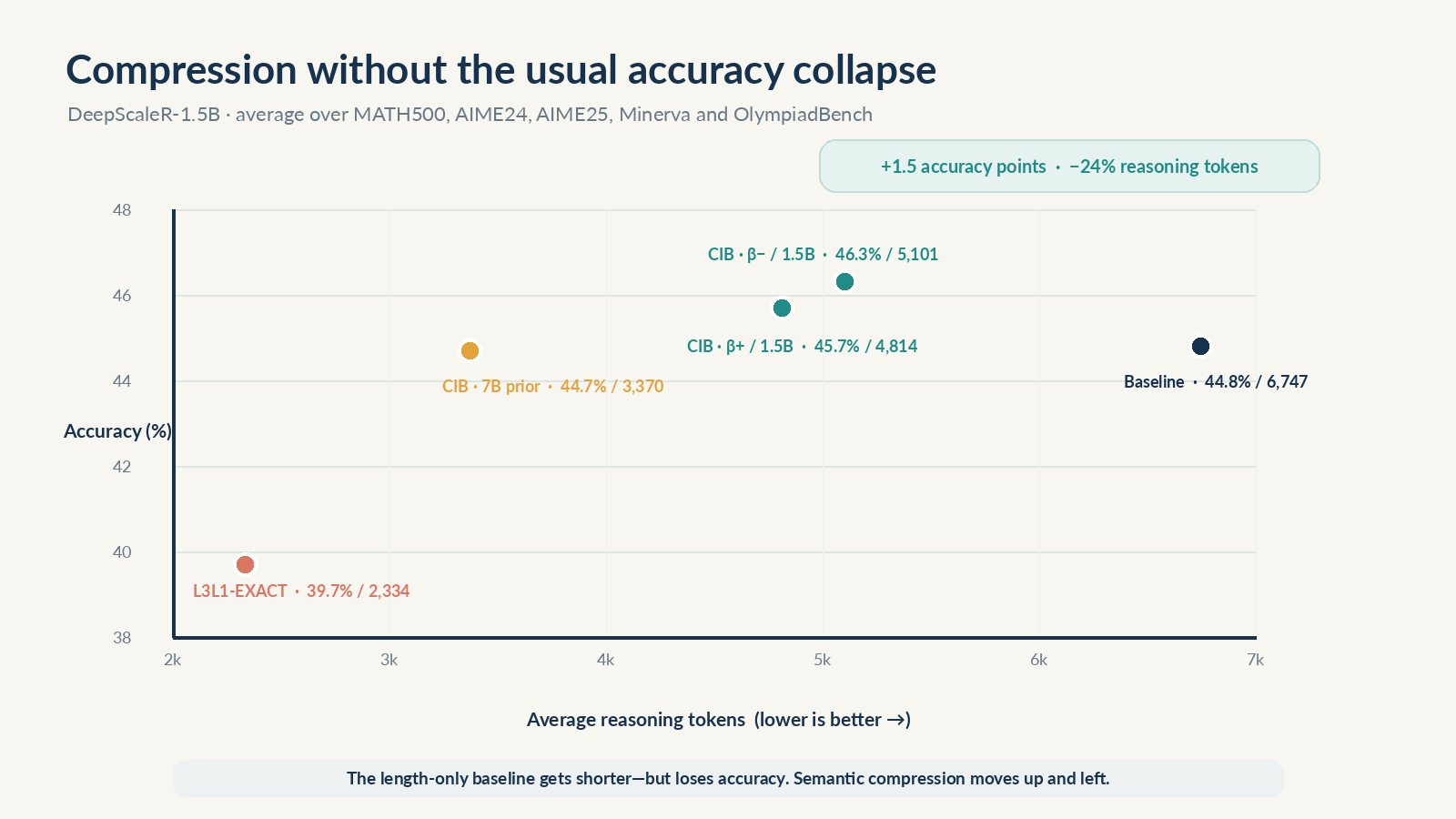
\[C(Z)=\sum_{t=1}^{T} -\log Q_\phi(z_t\mid z_{<t}).\]

Tokens are no longer equally expensive. Predictable, common tokens have low cost, while surprising tokens have higher cost. Crucially, this cost is balanced against the answer-accuracy reward. The model can therefore retain a costly but essential reasoning step when it helps produce the correct answer, while suppressing predictable, repetitive, or redundant reasoning. The figure from our paper illustrates the effectiveness of semantic compression.

Obtaining LLM post-training methods from CIB

Let’s go back to our original curiosity about the similarity of post-training methods. We introduce two changes to our bound: we use a conditional prior \(Q(z\mid x)\) instead of \(Q(z)\), and we replace mutual information with a general \(f\)-divergence:

\[\max_{\pi_\theta} \mathbb E_{(x,y)\sim P_{\textrm{true}},z\sim\pi_\theta(\cdot|x)} \left[ \log q_\theta(y\mid x,z) \right]-\beta \mathbb E_X D_{f} \big( \pi_\theta(z\mid X)\|Q(z\mid x)\big). \tag{5}\]

We can now obtain many familiar methods from this bound.

RLVR [1]: We can select \(\log q_\theta(y\mid x,z)\) such that the effective term in the objective is the verifier reward \(r_{\mathrm{VR}}(x,z)=\mathbf 1\{\widehat y(x,z)=y\}\). The parameter \(\beta\) controls whether we add budget forcing [6]. We typically sample on-policy from the model we are optimizing.

RLAIF [2]: We can select \(\log q_\theta(y\mid x,z)\) to reflect the AI critic that scores the final answer: \(r_{\mathrm{AI}}(\widehat y(x,z))\). We typically sample on-policy from the model we are optimizing.

OPD [3]: In OPD, the student generates the states on-policy: \(z\sim\pi_\theta(\cdot\mid x).\) A teacher provides a distribution \(q_T(z_t\mid x,z_{<t}).\) A canonical token-level OPD objective is:

\[\min_\theta \mathbb E_{x,z\sim\pi_\theta} \left[ \sum_{t=1}^{T} D_{f} \left( q_T(\cdot\mid x,z_{<t}) \| \pi_\theta(\cdot\mid x,z_{<t}) \right) \right].\]

Different choices of \(f\) give the forward or reverse KL divergence. This is a special case of the generalized conditional information bottleneck presented above.

SFT: Suppose the dataset contains demonstrations \((x,z^*).\) Ordinary SFT minimizes

\[\mathcal L_{\mathrm{SFT}} = -\mathbb E_{(x,z^*)\sim\mathcal D} \log \pi_\theta(z^*\mid x).\]

Equivalently,

\[\max_\theta \mathbb E_{(x,z^*)\sim\mathcal D} \log\pi_\theta(z^*\mid x).\]

If we introduce the empirical demonstration distribution \(Q_{\mathcal D}(z\mid x)\), then:

\[\mathbb E_{x,z\sim Q_{\mathcal D}} \log\pi_\theta(z\mid x) = -H(Q_{\mathcal D}) - \mathbb E_x D_{\mathrm{KL}} (Q_{\mathcal D}(\cdot\mid x) \| \pi_\theta(\cdot\mid x)).\]

Thus SFT is the offline analogue of distillation: the data distribution plays the role of the teacher. This can also be obtained from the generalized bottleneck formulation using off-policy sampling and the forward KL divergence.

Final words

The conditional information bottleneck framework provides a general way of thinking about post-training of reasoning models. It accommodates different sampling distributions and provides a framework for choosing a prior \(Q\) to control minimality and a sufficiency signal to measure task performance. The choice of \(\beta\) controls the compression rate, and we have shown in our experiments that the compression rate can be controlled smoothly with \(\beta\) [5]. RLVR, RLAIF, SFT, OPD, and self-distillation [4] can all be represented within a generalized variational CIB framework, in which post-training specifies a sufficiency functional and an information reference, while on-policy versus offline training specifies the trajectory distribution on which the functional is evaluated.

References

1. Shao, Z. et al.
   DeepSeekMath: Pushing the Limits of Mathematical Reasoning in Open Language Models. 2024.

2. Lee, H. et al.
   RLAIF: Scaling Reinforcement Learning from Human Feedback with AI Feedback. 2023.

3. Song, M. & Zheng, M.
   A Survey of On-Policy Distillation for Large Language Models. 2026.

4. Zhao, S. et al.
   Self-Distilled Reasoner: On-Policy Self-Distillation for Large Language Models. ICML 2026.

5. Massoli, F. V., Kuzmin, A., & Behboodi, A.
   Reasoning as Compression: Unifying Budget Forcing via the Conditional Information Bottleneck. NeurIPS 2026.

6. Aggarwal, P. & Welleck, S.
   L1: Controlling How Long a Reasoning Model Thinks With Reinforcement Learning. 2025.

7. Broome, J.
   Normativity, Rationality, and Reasoning: Selected Essays. Oxford University Press, 2021.

8. Tishby, N., Pereira, F. C., & Bialek, W.
   The Information Bottleneck Method. 1999.

9. Shwartz-Ziv, R. & Tishby, N.
   Opening the Black Box of Deep Neural Networks via Information. 2017.

10. Wei, J. et al.
    Chain-of-Thought Prompting Elicits Reasoning in Large Language Models. NeurIPS 2022.

11. Alemi, A. A., Fischer, I., Dillon, J. V., & Murphy, K.
    Deep Variational Information Bottleneck. ICLR 2017.